How Wrong is Too Wrong?

This is a crosspost from the Tensara blog.

For context, I help run Tensara, a competitive GPU programming platform with Somesh, Soham, and Harmya. If you haven't heard of it before, the gist is to compete to write the fastest GPU kernel for a given mathematical workload (GEMM, Conv, Attention, etc).

A major part of making this platform work is building robust verification + benchmarking harnesses for our problems. This post is about the former: what it even means to “verify” floating-point GPU kernels, and our efforts to make our acceptance criteria more principled than "ehh rtol=1e-3 seems fine.”

Each Tensara problem is defined by a reference solution $f$: a PyTorch implementation of the semantics of the problem. Let's represent the user submissions by $g$. Given the appropriate inputs $x$ as defined by the problem, we compute a reference output: $y = f(x)$ and a submission output: $w = g(x)$. We then decide whether to accept the submission by comparing $y$ and $w$.

We use torch.allclose, which checks the elementwise inequality

where $a$ is atol (absolute tolerance) and $r$ is rtol (relative tolerance). The core problem is that we have to pick these bounds -- and if done by hand, they can feel arbitrary. This post is about choosing $a$ and $r$ in a way that's (1) justifiable and (2) stable.

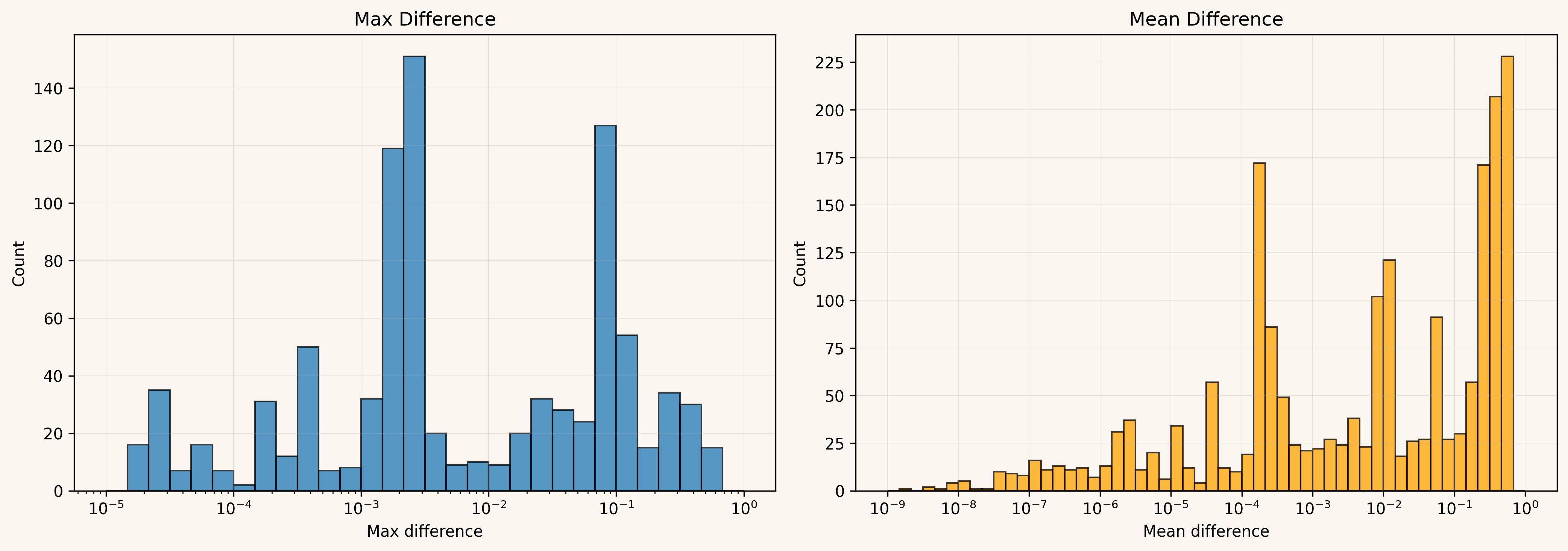
This is a distribution of the mean and max absolute differences across wrong submissions (filtered to those with mean/max difference < 1). Even among wrong submissions, the errors are often tiny: maximum differences frequently fall in the range $[10^{-5}, 10^{-3}]$, while mean differences reach down to $10^{-9}$, with many below $10^{-4}$.

Why should a submission that’s $10^{-6}$ away be rejected? Why should it be accepted?

Rather than answer those case-by-case with hand-picked tolerances for every problem, we chose to make a general explicit policy decision of the "lower bound of correctness".

A submission should not be able to pass if it performs the entire computation in a strictly lower-precision regime than intended.

Concretely, if the intended correctness is float32 then a solution that simply runs the whole workload in float16 (or worse) should not pass the float32 correctness check. This fits in well with our plans to add lower precision regimes for problems (..soon?), as it lets us make the intended precision target explicit and enforce clear boundaries between solution sets across those modes.

The nice thing about having this explicit lower bound of correctness is that we can turn it into something quantitative. Let's say we have $T$ testcases with inputs $\mathbf{x}^{(1)}, \mathbf{x}^{(2)}, \ldots \mathbf{x}^{(T)}$ for our problem. For each testcase $\mathbf{x}^{(t)}$, we first compute the reference output:

Next, we construct a corresponding “bad” output $\mathbf{z}^{(t)}$ by forcing a fully lower-precision implementation in PyTorch after casting the inputs down. The details can vary based off the problem, but the intent is to make $\mathbf{z}^{(t)}$ as a representative output that we do not want to accept as close enough to $\mathbf{y}^{(t)}$. This gives us a dataset of pairs:

that we want our eventual tolerances to reject.

Let's start with defining tensors $\mathbf{d}$ and $\mathbf{s}$ for each pair $\left(\mathbf{z}^{(t)}, \mathbf{y}^{(t)}\right) \in \mathcal{B}$:

We can then write our torch.allclose() constraint as:

$a$ and $r$ both shape the same acceptance bound. $a$ matters most when $\mathbf{s}_i$ is small, and $r$ matters most when $\mathbf{s}_i$ is large, so choosing them independently is hard to reason about.

So we (heuristically) pick a typical scale $s' = \mathrm{median}(\mathbf{s})$. We then pin the ratio by enforcing $a = r \cdot s'$. That collapses the problem to one free variable $r$, with the absolute/relative tradeoff $s'$ set by the problem’s numerics rather than by hand.

Plugging $a = r \cdot s'$ back into the constraint:

Let's define

Intuitively, $\rho_i$ is the per-element required $r$ for that entry to pass under the coupled rule $a = r\cdot s'$.

All that’s left is choosing a single $r$ from the per-element requirements $\rho_i$. Taking the max would make the tolerance hinge on one worst-case element, which can be fairly noisy across different problem types. So we soften it: we pick a percentile (we used 75%) and choose $r_t$ so that roughly three quarters of the entries still satisfy the bound (equivalently, one quarter of entries fail). Then we set $a_t = r_t \cdot s'$.

Now we have one pair $(a_t, r_t)$ per testcase. We still need one global pair, and we don’t want it to be decided by a single outlier seed. So we score each testcase by $m_t = \max(a_t, r_t)$, sort by $m_t$, and take the median testcase.

That testcase’s $(a_t, r_t)$ becomes our global $(a, r)$.

This still isn’t perfect, it’s a heuristic, but it’s much more grounded than what we had. There are a few obvious upgrades:

• Today we only anchor on bad pairs. If we can systematically generate near-boundary good pairs too, this turns into a clean separation problem (pick $r$ with margin).
• Input distributions matter. Keeping ranges small helps, but a better approach is probably multiple regimes (typical + stress) with explicit intent.
• Longer term we want explicit precision rungs (fp32, bf16/fp16, fp8, etc). Then verification is just making sure each tier doesn’t bleed into the next, and we can label what tier a submission effectively falls into.
• The median and percentile choices still have some arbitrariness. There’s room to analyze which kinds of workloads are sensitive to these knobs (and why), and which ones are basically indifferent to make a more informed choice.

For now, these changes put us in a better place to innovate in this context, with fewer ad hoc decisions along the way.

If you’re working on floating-point verification, benchmarks, or GPU-kernel weirdness and you made it this far, we’d probably get along. Reach out!