Norm Balancing Optimizers

TL;DR: Balancing row and column-wise update magnitudes alone can reproduce a surprising share of Muon’s performance. Across a CNN, an MLP, and a small transformer, this lightweight norm-balancing step often matches AdamW and sometimes closes much of the gap to Muon, without explicit orthogonalization and without any extra variance/second-moment buffers. These results suggest norm balancing may be a simple, useful source of optimizer stability worth studying on its own.

Preconditioning is an important part of the deep learning optimizer puzzle. Adaptive optimizers like AdamW¹ rescale each coordinate using a running estimate of the gradient’s second moment. Matrix-aware methods such as Shampoo² and SOAP³ go further by explicitly modeling the geometry of matrix-valued parameters through structured preconditioners.

Recent work on Muon⁴ takes a different but related path: rather than estimating curvature, it directly reshapes the update matrix itself, approximately orthogonalizing momentum updates via Newton–Schulz before applying them. This preconditioning of the momentum updates is conceptually similar⁵ to Shampoo with its EMAs disabled: both project updates toward semi-orthogonal matrices.

Muon’s update transform mixes two geometric effects. It pushes momentum updates toward being semi-orthogonal along the shorter axis (via approximate orthogonalization), while also making the update closer to unit-norm per row/column. This post isolates the second effect. Concretely: how much stability and performance can we recover by only balancing row/column update magnitudes, without enforcing orthogonality?

We study a stripped-down Muon variant that keeps the same momentum matrix $M_t$, but replaces Newton–Schulz orthogonalization with a lightweight axis-balancing transform. For this post, let's call this variant BAM: Balanced Axis Momentum. Concretely, BAM applies a Sinkhorn-Knopp inspired process called SinkNorm, which alternates row-wise and column-wise $\ell_2$ normalization for $K$ steps:

def sinknorm(M, K: int, eps: float = 1e-7):
    m, n = M.shape[-2], M.shape[-1]
    col_first = (m > n)  # ensures we end on the smaller dimension
    X = M
    for _ in range(K):
        if col_first:
            X = X / (torch.linalg.vector_norm(X, 2, dim=-2, keepdim=True) + eps) # cols 
            X = X / (torch.linalg.vector_norm(X, 2, dim=-1, keepdim=True) + eps) # rows
        else:
            X = X / (torch.linalg.vector_norm(X, 2, dim=-1, keepdim=True) + eps) # rows
            X = X / (torch.linalg.vector_norm(X, 2, dim=-2, keepdim=True) + eps) # cols
    return X

To compare these transforms directly, we take a matrix $M_0 \in \mathbb{R}^{1024\times 1024}$ and apply SinkNorm (BAM) with $K = 1$ or 3 steps of Newton-Schulz, and plot (a) the singular-value spectrum and (b--c) the ratios of row/column $\ell_2$ norms to their median norms:

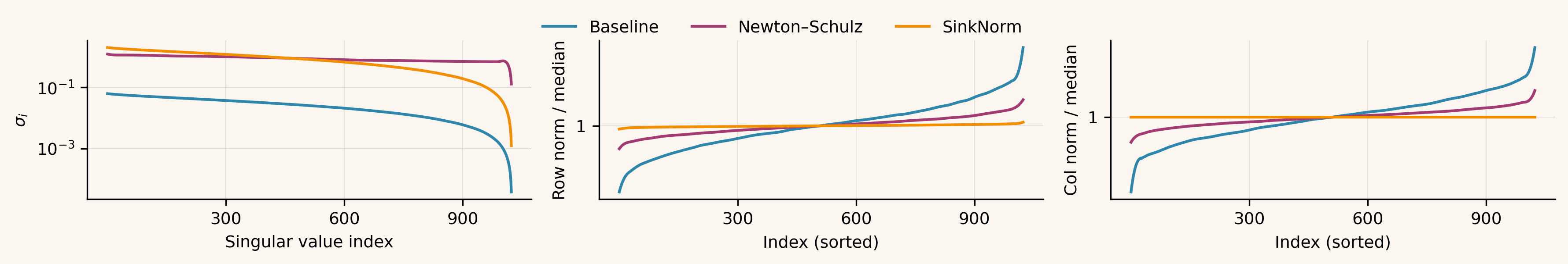
SinkNorm largely preserves the spectrum shape and mainly rescales to equalize row/column norms (i.e. condition number remains roughly the same). Newton–Schulz pushes the spectrum toward a much flatter, near-unit singular-value distribution while also improving row/column norm balance (though with noticeably more spread than SinkNorm).

Experiments

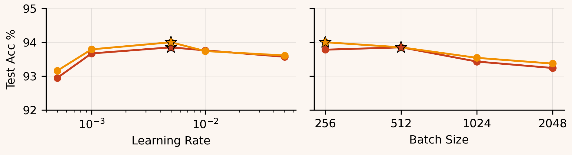
We compare AdamW, Muon, and BAM on three settings: a CNN (ResNet-18⁶ on CIFAR-10⁷), an MLP (a 4-layer MLP on CIFAR-10), and a small transformer (nanoGPT⁸ on FineWeb⁹). In all cases, we fix the dataset, architecture, and training budget. To isolate the effect of the matrix-update transform, we use the same parameter split in every run: non-2D parameters are always optimized with AdamW using fixed hyperparameters, while hidden 2D weight matrices use AdamW, Muon, or BAM.

For each experiment, we sweep the learning rate $\eta$ and batch size $B$ (effective token-batch size for nanoGPT). Each plotted point reports the best final metric at fixed $\eta$ (left) or fixed $B$ (right), maximizing over the remaining sweep dimensions. Full sweep grids and parameter-group definitions are provided here.

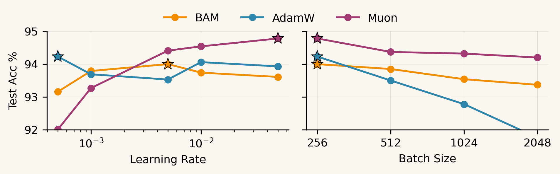
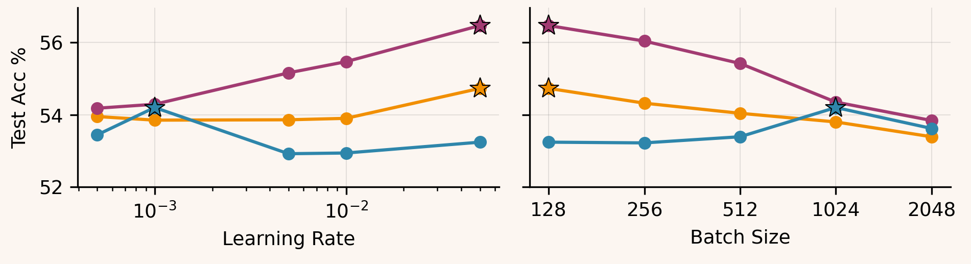
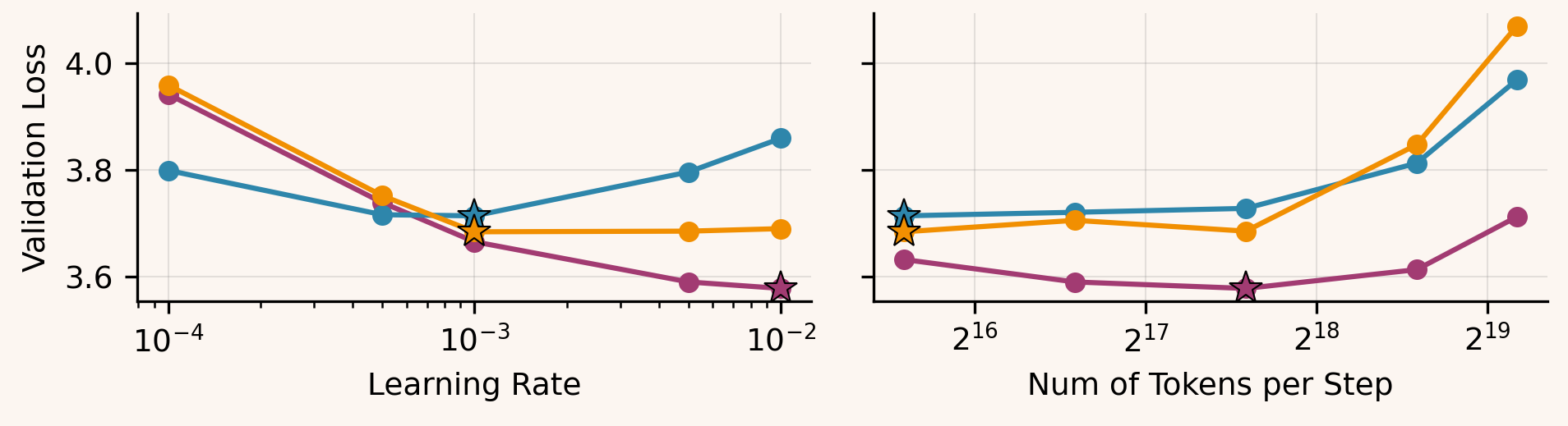
The same pattern shows up across settings. Muon achieves the best peak performance and tends to keep improving as $\eta$ increases (its optimum shifts toward larger $\eta$). BAM typically peaks at a more moderate $\eta$ than Muon: it looks fairly flat in the MLP, and in nanoGPT it bottoms out around $\eta \approx 10^{-3}$ before largely plateauing. AdamW, in contrast, generally peaks at smaller $\eta$ and is the first to degrade as $\eta$ grows.

As the batch size increases, the behavior becomes task-dependent. On ResNet-18, AdamW exhibits the strongest large-$B$ degradation, while BAM stays much closer to Muon's robustness. For the MLP, all three methods remain fairly stable across $B$, with only modest differences and a small crossover around $B = 1024$. For nanoGPT, the largest-token regime is the main outlier: Muon stays best, while BAM and AdamW both deteriorate sharply as tokens/step grow, with BAM drifting toward (and slightly above) AdamW at the extreme.

For additional context, we track two update-geometry diagnostics: the update’s distance to orthogonality (defined here) $\delta_{\perp}$ and the row/column $\ell_2$ coefficient of variation (the standard deviation of $\ell_2$ norms divided by their mean). These are computed on a hidden weight matrix: the MLP’s second linear layer, a convolutional layer in ResNet’s second stage, and (for nanoGPT) the first block’s self-attention QKV projection. We log these across training steps for the best-performing run within each (model, optimizer) pair:

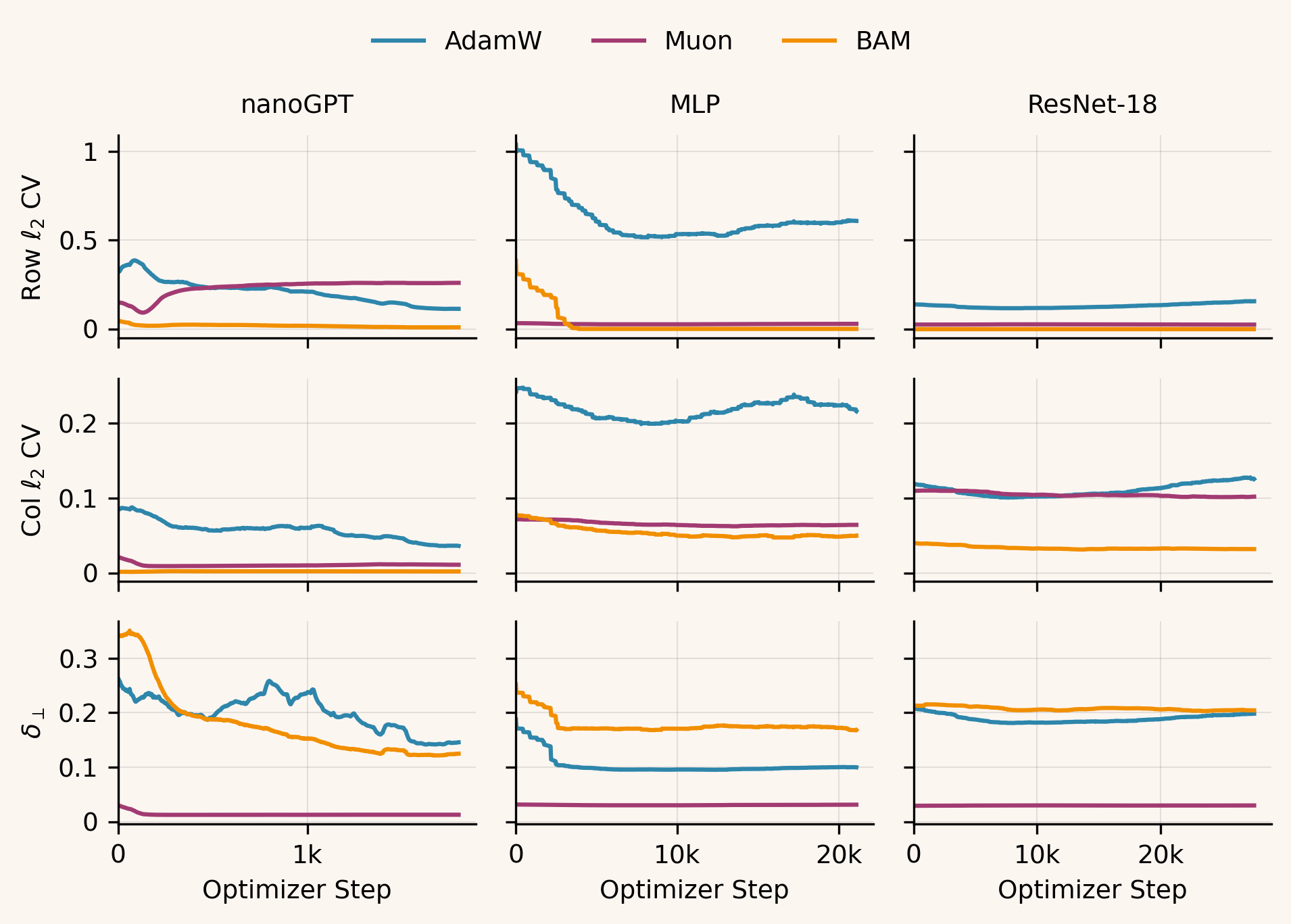
Muon drives $\delta_\perp$ down throughout training, while BAM remains close to AdamW; however, BAM matches Muon in reducing row/column CV, both far below AdamW across models.

Discussion

These experiments suggest that Muon’s benefits are not solely tied to spectrum flattening or approximate orthogonalization. A large fraction can be recovered by a much simpler geometric intervention of balancing row- and column-wise update magnitudes, even when the singular-value profile remains largely unchanged.

That said, we only evaluate moderate-scale models under fixed training budgets. The nanoGPT largest-token regime is a concrete case where BAM appears to lose its earlier advantage, hinting that spectrum shaping (or something correlated with it) may matter more in higher batch regimes.

Overall, these results are mainly meant as a lens: lightweight geometric control can already go a long way, and it provides a simpler way to reason about what Muon is buying beyond spectrum shaping.

Additional Experiments

Beyond the core sweeps, we ran a handful of smaller experiments to probe where the mechanisms might break. These are not as fully tuned or exhaustive, but they helped surface a few concrete questions worth following up on.

One-Axis Balancing

We tested a simplified variant of BAM (let's call it HalfBAM) that only normalizes the update along the shorter axis (i.e., enforces a shortest-axis ℓ₂ normalization) rather than alternating row/column normalization to balance both axes.

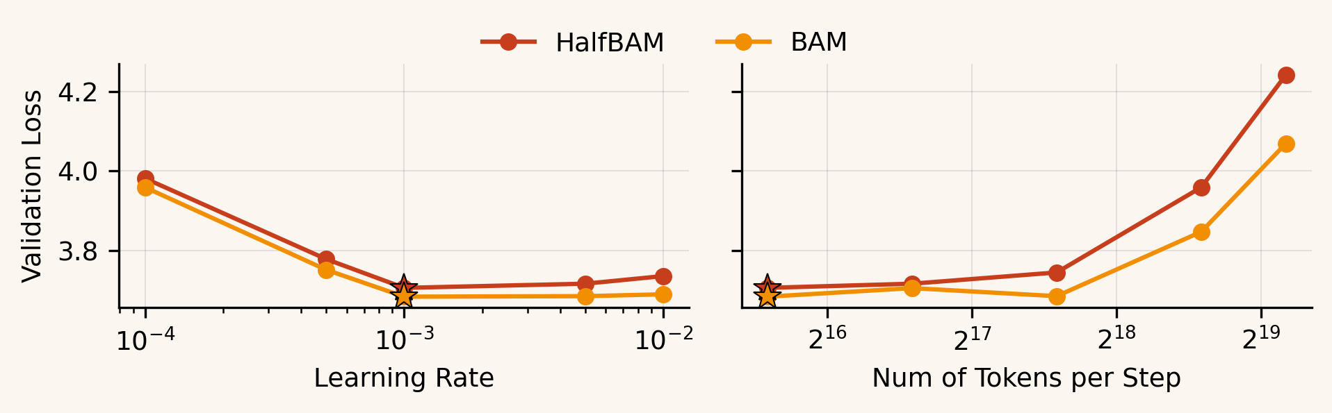
HalfBAM tracks BAM closely on the 4-layer MLP and ResNet-18 across learning rates and batch sizes, suggesting those models don’t strongly depend on balancing the longer axis.

In nanoGPT, the gap widens -- especially at higher tokens/step. Is this just a scale/throughput effect, or does attention/MLP block structure make transformers uniquely sensitive to long-axis imbalance?

SVD-based Orthogonalization

We also tested the opposite extreme geometric control: what if we take Muon’s approximate orthogonalization step and make it exact? We implemented an “SVD Muon” reference optimizer with the same high-level structure as Muon, but replacing the Newton–Schulz iteration with explicit SVD orthogonalization: compute $M = U \Sigma V^\top$ and set $M = UV^\top$ (discarding $\Sigma$).

In the MLP and ResNet-18 sweeps, exact SVD projection typically underperforms Muon’s Newton–Schulz approximation:

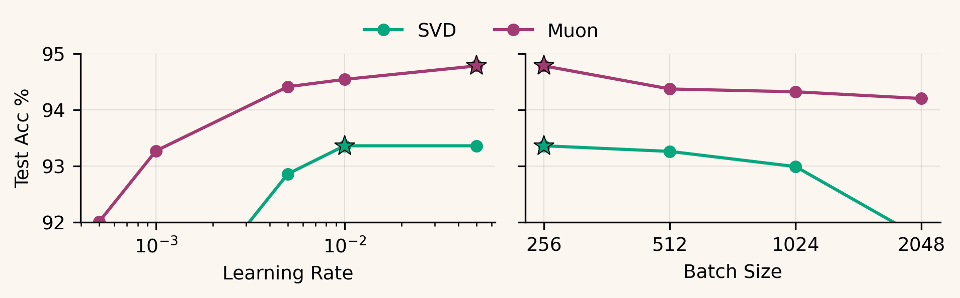
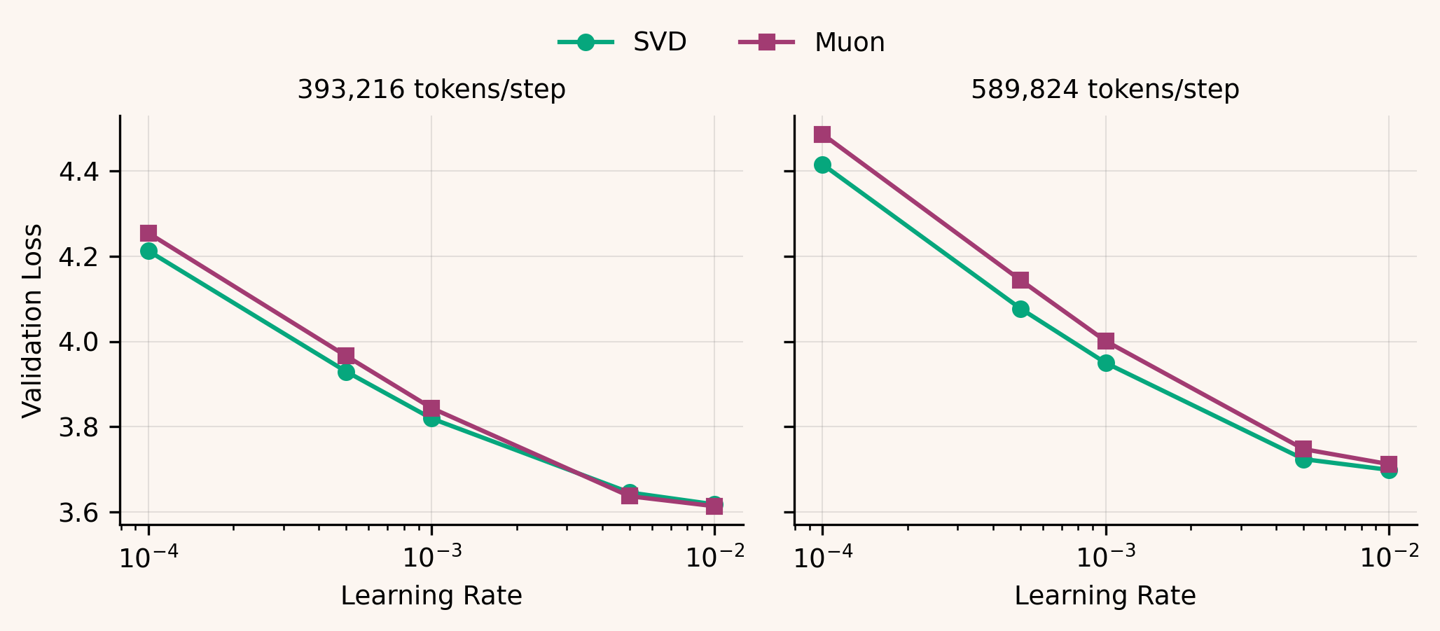
However, in the nanoGPT regime (393k and 589k tokens/step), SVD Muon closely matches and sometimes slightly improves on Muon:

More investigation is needed to understand where this crossover comes from: at what point does making the projection exact stop paying off (model scale, tokens/step, matrix shapes)?

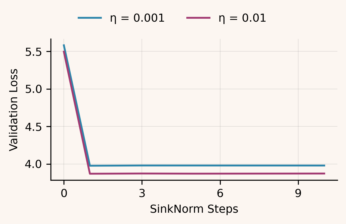
Ablation on SinkNorm iterations

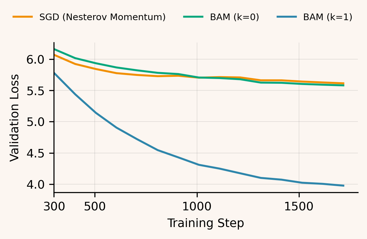
We ablated the number of SinkNorm iterations $k$ used in BAM, including $k=0$ as a no-balancing baseline. The effect saturates immediately: $k=1$ captures essentially the full gain, with larger $k$ yielding negligible improvement across learning rates. We therefore use $k=1$ in all main experiments. Notably, $k=0$ reduces to SGD with Nesterov momentum on these parameters, and its validation curve closely matches a SGD with Nesterov momentum run.

Future Work

There are a few obvious next steps. One is to test how far norm balancing scales by testing on larger models, more training steps, and more extreme batch sizes. Another is to probe the underlying mechanism more directly by tracking what changes in the training dynamics (beyond the simple geometry metrics here) when we balance axes vs when we also reshape the spectrum. Finally, it would be useful to connect these empirical regimes to a theoretical picture of why axis balancing helps.

These results suggest that surprisingly simple geometric interventions can already go a long way. We hope this analysis serves as a starting point for further investigation into this line of questioning. Our code for the experiments is available here.

Acknowledgments

We would like to thank Prof. Joseph Campbell for helpful discussion and feedback on this work. We also thank Keller Jordan for his work on running the CIFAR-10 and nanoGPT speedruns.

Citation

While the paper is not yet published, you can cite this work as:

@article{bam2026,
  title   = {Norm Balancing Optimizers},
  author  = {Mangla, Sarthak and Gurung, Abel},
  year    = {2026},
  month   = {February},
  url     = "https://sarthakmangla.com/blog/bam/"
}

References

1. Loshchilov, I. and Hutter, F. (2019) "Decoupled Weight Decay Regularization". ↩
2. Gupta, V., Koren, T. and Singer, Y. (2018) "Shampoo: Preconditioned Stochastic Tensor Optimization". ↩
3. Vyas, N. et al. (2025) "SOAP: Improving and Stabilizing Shampoo using Adam". ↩
4. Jordan, K. et al. (2024) "Muon: An optimizer for hidden layers in neural networks". ↩
5. Bernstein, J. and Newhouse, L. (2024) "Old Optimizer, New Norm: An Anthology". ↩
6. He, K. et al. (2015) "Deep Residual Learning for Image Recognition". ↩
7. Krizhevsky, A. and Hinton, G. (2009) "Learning multiple layers of features from tiny images". ↩
8. Karpathy, A. (2022) "nanoGPT". ↩
9. Penedo, G. et al. (2024) "The FineWeb Datasets: Decanting the Web for the Finest Text Data at Scale". ↩

Appendix

Orthogonality Gap $\delta_\perp$

For a matrix $M\in\mathbb{R}^{r\times c}$, let $d=\min(r,c)$. This metric measures how close the vectors along the shorter axis of $M$ are to being orthonormal after removing simple scale differences. Let $A\in\mathbb{R}^{d\times \max(r,c)}$ be the matrix whose rows are the vectors of $M$ along its shorter axis (i.e., $A=M$ if $r\le c$, else $A=M^\top$). Normalize each row to unit $\ell_2$ norm:

Form the Gram matrix of these normalized vectors,

If the normalized vectors are perfectly orthonormal, then $G=I_d$. The orthogonality gap is the normalized Frobenius distance to identity:

Intuitively, $\delta_\perp(M)$ reflects the typical magnitude of off-diagonal correlations between normalized shorter-axis vectors. It is zero when they are exactly orthonormal, and increases as they become more aligned.

Parameter Groups + Hyperparameter Sweeps

Across experiments, we split parameters into a 2D group (matrix-valued weights) and a fixed-AdamW group (everything else). For all runs, we apply Muon/BAM/AdamW only to the 2D group, while training the remaining parameters with a fixed AdamW configuration.

ResNet-18: The 2D group consists of all convolution kernels inside residual blocks and shortcut paths (4D kernels reshaped to 2D), excluding the stem conv1.weight. The fixed-AdamW group includes conv1.weight, all BatchNorm parameters, and classifier parameters (linear.weight, linear.bias).

We sweep:

• batch size $B \in \{256,512,1024,2048\}$
• learning rate $\eta \in \{5\!\cdot\!10^{-4},10^{-3},5\!\cdot\!10^{-3},10^{-2},5\!\cdot\!10^{-2}\}$
• momentum $\beta$ (Muon/BAM) or $\beta_1$ (AdamW) in $\{0.9,0.95,0.99\}$.

We fix AdamW $\beta_2=0.999$; weight decay $10^{-3}$; linear LR decay to zero with no warmup. Non-2D parameters use AdamW with $\eta=10^{-3}$ and weight decay $10^{-3}$. We train for 100 epochs with label smoothing 0.2.

MLP: The 2D group contains fc2.weight and fc3.weight, while the fixed-AdamW group contains fc1.weight and fc4.weight.

We sweep:

• $B \in \{128,256,512,1024,2048\}$
• $\eta \in \{5\!\cdot\!10^{-4},10^{-3},5\!\cdot\!10^{-3},10^{-2},5\!\cdot\!10^{-2}\}$
• momentum $\beta$ or $\beta_1 \in \{0.9,0.95,0.99,0.999\}$
• weight decay in $\{0,10^{-1},10^{-2},10^{-3},10^{-4}\}$

We fix: AdamW $\beta_2=0.999$; linear LR decay to zero with no warmup. Non-2D parameters use AdamW with $\eta=10^{-4}$ and zero weight decay. We train for 50 epochs with no label smoothing.

nanoGPT: We train with a three-phase learning-rate schedule shared by all optimizers: 10% linear warmup from 0 to the base rate, a constant plateau whose duration is set by a swept stable fraction, and a cosine decay from the base rate down to $0.1\times$ the base rate. We sweep token batch size $B$ by varying gradient accumulation with fixed microbatch size $B_M=12$ and sequence length $L=1024$, so

The 2D group consists of all matrix weights in attention/MLP blocks (e.g., c_attn.weight, c_proj.weight, c_fc.weight). The fixed-AdamW group includes the token/position embeddings (wte, wpe), lm_head, and all non-2D parameters (biases and normalization parameters). We also modify the original nanoGPT implementation with a few modernization tweaks: QK norm, ReLU$^2$ in place of GELU, and zero-initialized residual projection matrices.

We sweep:

• token batch size $B \in \{49152,98304,196608,393216,589824\}$
• 2D learning rate $\eta \in \{10^{-4},5\!\cdot\!10^{-4},10^{-3},5\!\cdot\!10^{-3},10^{-2}\}$
• stable-plateau fraction in $\{0.0,0.3\}$

We fix Muon/BAM momentum $\beta=0.95$. Non-2D parameters use AdamW with $\eta=6\!\cdot\!10^{-4}$ and $(\beta_1,\beta_2)=(0.9,0.95)$. We use weight decay 0.1, gradient clipping 1.0, bf16 precision, and a 700M-token budget.